Basic usage
In this notebook, we demonstrate how to use FitMultiCell to interface the model development and simulation tool Morpheus with the parameter inference tool pyABC.
[1]:
import fitmulticell as fmc
import pyabc

import scipy as sp
import numpy as np
import pandas as pd
import os
import tempfile

%matplotlib inline
pyabc.settings.set_figure_params('pyabc')  # for beautified plots
[2]:
fmc.log.print_version()
Running FitMultiCell 0.0.7 with Morpheus 2.2.3, pyABC 0.11.11 on Python 3.7.5 at 2022-01-20 12-37.
Inference problem definition
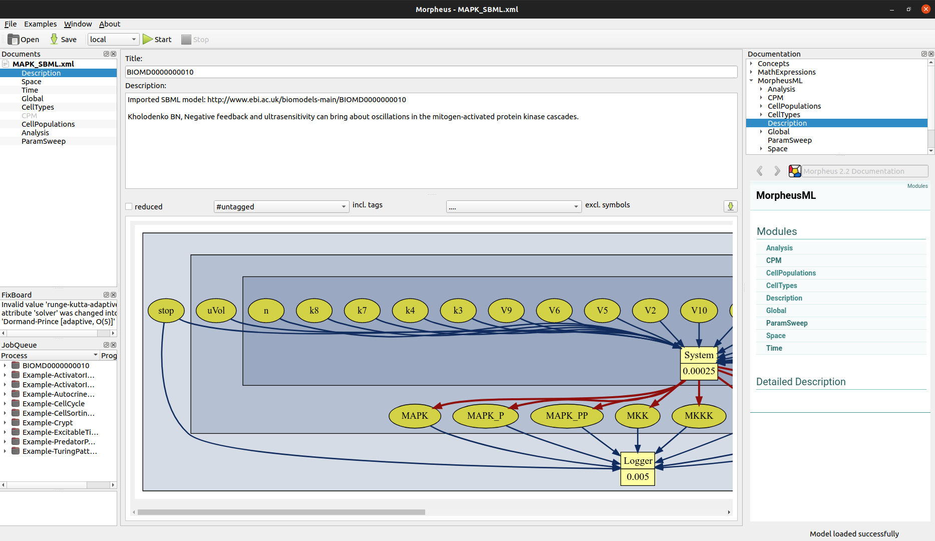
We consider the problem of fitting various parameters for a simple ODE model of MAPK signaling, taken from Morpheus’ built-in examples, with synthetic data. Model construction and refinement can be done via Morpheus’ GUI, see its homepage for tutorials and help.
[3]:
# model file
model_file = os.path.join("models", "MAPK_SBML.xml")

# run morpheus
# !morpheus-gui --url=$model_file

# display gui
from IPython.display import Image
Image("_static/morpheus_gui.png", width=800)
[3]:
The Morpheus model specification is contained in a single XML file, which can be read in by FitMultiCell via the MorpheusModel <fitmulticell.model.MorpheusModel> class. See the API documentation for configuration options, e.g. allowing to specify the Morpheus executable, summary statistics, and level of output. The default summary statistics are just the values logged in the “logger.csv” file generated by Morpheus.
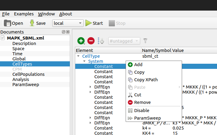
Assuming various of the model parameters to be unknown, we intend to infer them from observed data via pyABC. Therefore, we specify the mapping of parameter ids to XPaths in the model file. XPaths of model entities can be easily obtained via the Morpheus GUI “Copy XPath” context menu.
[4]:
Image("_static/morpheus_xpath.png", width=400)
[4]:
[5]:
# parameter mapping
par_map = {
    "V1": "./CellTypes/CellType/System/Constant[@symbol='V1']",
    "V2": "./CellTypes/CellType/System/Constant[@symbol='V2']",
    "k3": "./CellTypes/CellType/System/Constant[@symbol='k3']",
}

# Morpheus model
model = fmc.model.MorpheusModel(
    model_file=model_file,
    par_map=par_map,
    raise_on_error=False,
)
print(model)
MorpheusModel {
  name         : models/MAPK_SBML.xml
  par_map      : {'V1': "./CellTypes/CellType/System/Constant[@symbol='V1']", 'V2': "./CellTypes/CellType/System/Constant[@symbol='V2']", 'k3': "./CellTypes/CellType/System/Constant[@symbol='k3']"}
  sumstat      : None
  executable   : morpheus
}
A short check whether everything works, prior to the analysis, is usually useful.
[6]:
model.sanity_check()
FitMultiCell.Model INFO: Sanity check successful
Let us generate some dummy observed data from synthetic ground-truth parameters true_pars. The parameters we define here must correspond to Constants in the Morpheus XML file.
[7]:
true_pars = {'V1': 2.7, 'V2': 0.25, 'k3': 0.025}
limits = {key: (0.5 * val, 2 * val) for key, val in true_pars.items()}

# generate data
observed_data = model.sample(true_pars)
print(observed_data.keys())
dict_keys(['time', 'cell.id', 'MAPK', 'MAPK_P', 'MAPK_PP', 'MKK', 'MKK_P', 'MKK_PP', 'MKKK', 'MKKK_P'])
As usual, we have to define a prior for our parameters.
[8]:
prior = pyabc.Distribution(
    **{
        key: pyabc.RV("uniform", lb, ub - lb)
        for key, (lb, ub) in limits.items()
    }
)
Also, we have to define a distance which computes a scalar value quantifying the discrepancy of generated and observed data. Note that also this step can be customized, e.g. for arbitrary summary statistics. Here, we use a simple L1 distance between selected outputs.
[9]:
def distance(val1, val2):
    d = np.sum(
        [
            np.sum(np.abs(val1[key] - val2[key]))
            for key in ['MAPK_P', 'MKK_P']
        ]
    )
    return d
Running the ABC inference
Now, we are able to run our ABC analysis. See the pyABC documentation for configuration options, e.g. regarding parallelization, distances, thresholds, or proposal distributions.
[10]:
abc = pyabc.ABCSMC(model, prior, distance, population_size=100)
db_path = "sqlite:///" + os.path.join(tempfile.gettempdir(), "test.db")
abc.new(db_path, observed_data)
ABC.Sampler INFO: Parallelize sampling on 12 processes.
ABC.History INFO: Start <ABCSMC id=1, start_time=2022-01-20 12:38:11>
[10]:
<pyabc.storage.history.History at 0x7f969c715190>
[11]:
history = abc.run(max_nr_populations=5)
ABC INFO: Calibration sample t = -1.
ABC INFO: t: 0, eps: 1.42432419e+04.
ABC INFO: Accepted: 100 / 186 = 5.3763e-01, ESS: 1.0000e+02.
ABC INFO: t: 1, eps: 1.14215269e+04.
ABC INFO: Accepted: 100 / 235 = 4.2553e-01, ESS: 7.9988e+01.
ABC INFO: t: 2, eps: 8.96405597e+03.
ABC INFO: Accepted: 100 / 237 = 4.2194e-01, ESS: 8.9190e+01.
ABC INFO: t: 3, eps: 6.12055219e+03.
ABC INFO: Accepted: 100 / 178 = 5.6180e-01, ESS: 8.2634e+01.
ABC INFO: t: 4, eps: 4.79957563e+03.
ABC INFO: Accepted: 100 / 199 = 5.0251e-01, ESS: 8.6064e+01.
ABC INFO: Stop: Maximum number of generations.
ABC.History INFO: Done <ABCSMC id=1, duration=0:00:40.425872, end_time=2022-01-20 12:38:51>
Visualization and analysis
The history file contains the analysis results. We can use pyABC’s visualization routines to analyse the result.
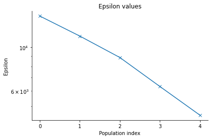
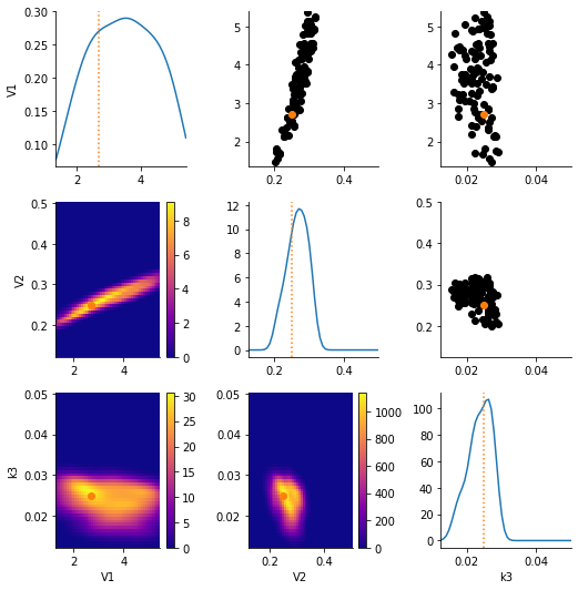
[12]:
pyabc.visualization.plot_epsilons(history)
pyabc.visualization.plot_kde_matrix_highlevel(history, limits=limits, refval=true_pars);