Count Active infected Cell
In this notebook, we will try to count the number of CC contributor in hexagonal grid.
The CC contributor cells are those who contribute to cell-to-cell transmission.
To do so, we will use a function called get_count_cc_contributors_alltp. This function takes the Morpheus log output as pd.df, the field of interest that contain the cell information, the list of cell types that are member of the cluster, the time interval of which we want to count the CC contributor cells (optional), the time step (optional), and the time symbol, as specified in the Morpheus model. The output will be a dictionary with time points as a keys, and the count of the CC
contributor cells as values.
Let try to use the function now, but before we start, let’s define some required parameters. First, let’s create a sample logger file in a CSV format:
[14]:
import csv
import tempfile
import os

full_path=os.path.join(tempfile.gettempdir(), "logger.csv")

csvfile=open(full_path,'w', newline='')
obj=csv.writer(csvfile, delimiter='\t')
obj.writerow(['t', 'cell.id', 'RNA_concentration', 'infection'])
obj.writerow(['0', '1', '0.1' ,'1'])
obj.writerow(['0', '2', '0.2' ,'1'])
obj.writerow(['0', '3', '0.3' ,'0'])
obj.writerow(['0', '4', '0.4' ,'1'])
obj.writerow(['0', '5', '0.5' ,'1'])
obj.writerow(['0', '6', '0.6' ,'0'])
obj.writerow(['0', '7', '0.7' ,'0'])
obj.writerow(['0', '8', '0.8' ,'0'])
obj.writerow(['0', '9', '0.9' ,'0'])
obj.writerow(['0', '10', '0.9' ,'0'])
obj.writerow(['0', '11', '0.9' ,'0'])
obj.writerow(['0', '12', '0.9' ,'0'])
obj.writerow(['0', '13', '0.9' ,'0'])
obj.writerow(['0', '14', '0.9' ,'0'])
obj.writerow(['0', '15', '0.9' ,'0'])
obj.writerow(['0', '16', '0.9' ,'0'])
obj.writerow(['0', '17', '0.9' ,'1'])
obj.writerow(['0', '18', '0.9' ,'0'])
obj.writerow(['0', '19', '0.9' ,'1'])

obj.writerow(['1', '1', '0.1' ,'1'])
obj.writerow(['1', '2', '0.2' ,'1'])
obj.writerow(['1', '3', '0.3' ,'0'])
obj.writerow(['1', '4', '0.4' ,'1'])
obj.writerow(['1', '5', '0.5' ,'1'])
obj.writerow(['1', '6', '0.6' ,'0'])
obj.writerow(['1', '7', '0.7' ,'0'])
obj.writerow(['1', '8', '0.8' ,'1'])
obj.writerow(['1', '9', '0.9' ,'1'])
obj.writerow(['1', '10', '0.9' ,'0'])
obj.writerow(['1', '11', '0.9' ,'0'])
obj.writerow(['1', '12', '0.9' ,'0'])
obj.writerow(['1', '13', '0.9' ,'1'])
obj.writerow(['1', '14', '0.9' ,'0'])
obj.writerow(['1', '15', '0.9' ,'1'])
obj.writerow(['1', '16', '0.9' ,'1'])
obj.writerow(['1', '17', '0.9' ,'1'])
obj.writerow(['1', '18', '0.9' ,'0'])
obj.writerow(['1', '19', '0.9' ,'1'])


csvfile.close()
The data above describe a hexagonal grid with two types of cell, infected or not infected. The infected cell will have infection value = 1. The data describe the grid in two time steps (0 and 1).
the hexagonal grid we look like this:
Time_step=0:
           / \     / \     / \
         /     \ /     \ /     \
        | inf=1 | inf=0 | inf=1 |
        |c-id=17|c-id=18|c-id=19|
       / \     / \     / \     / \
     /     \ /     \ /     \ /     \
    | inf=0 | inf=0 | inf=0 | inf=0 |
    |c-id=13|c-id=14|c-id=15|c-id=16|
   / \     / \     / \     / \     / \
 /     \ /     \ /     \ /     \ /     \
| inf=0 | inf=0 | inf=0 | inf=0 | inf=0 |
|c-id=8 |c-id=9 |c-id=10|c-id=11|c-id=12|
 \     / \     / \     / \     / \     /
   \ /     \ /     \ /     \ /     \ /
    | inf=1 | inf=1 | inf=0 | inf=0 |
    |c-id=4 |c-id=5 |c-id=6 |c-id=7 |
     \     / \     / \     / \     /
       \ /     \ /     \ /     \ /
        | inf=1 | inf=1 | inf=0 |
        |c-id=1 |c-id=2 |c-id=3 |
         \     / \     / \     /
           \ /     \ /     \ /
Time_step=1:
           / \     / \     / \
         /     \ /     \ /     \
        | inf=1 | inf=0 | inf=1 |
        |c-id=17|c-id=18|c-id=19|
       / \     / \     / \     / \
     /     \ /     \ /     \ /     \
    | inf=1 | inf=0 | inf=1 | inf=1 |
    |c-id=13|c-id=14|c-id=15|c-id=16|
   / \     / \     / \     / \     / \
 /     \ /     \ /     \ /     \ /     \
| inf=1 | inf=1 | inf=0 | inf=0 | inf=0 |
|c-id=8 |c-id=9 |c-id=10|c-id=11|c-id=12|
 \     / \     / \     / \     / \     /
   \ /     \ /     \ /     \ /     \ /
    | inf=1 | inf=1 | inf=0 | inf=0 |
    |c-id=4 |c-id=5 |c-id=6 |c-id=7 |
     \     / \     / \     / \     /
       \ /     \ /     \ /     \ /
        | inf=1 | inf=1 | inf=0 |
        |c-id=1 |c-id=2 |c-id=3 |
         \     / \     / \     /
           \ /     \ /     \ /
where inf represents the infection and c-id represent the cell ID.
So, let’s define the required parameters and run the function. The field of interest will be infection:
[15]:
field_of_interest='infection'
We also need to define the list of the cell types that are members of the cluster formation. In this simple example, we consider a cell to be infected only if it has a value of 1.
[16]:
cluster_cell_types=[1]
Finally, we will specify the time_interval, and the time_symbol, both as specified in the Morpheus model.
[17]:
t_interval=[0,1]
t_symbol='t'
After defining all the required parameter, let’s run the function. But before that, let’s import the function’s library. Don’t forget to install the package first.
[18]:
import fitmulticell.sumstat.hexagonal_cluster_sumstat as css
We also need to import util library form fitmulticell to read the CSV file as pandas df
[19]:
import fitmulticell.util as util
No, we will read the CSV file using the tsv_to_df function form the external library
[20]:
logger_file = util.tsv_to_df("/tmp")
Let’s see how the logger_file loks like
[21]:
logger_file
[21]:
| t | cell.id | RNA_concentration | infection | |
|---|---|---|---|---|
| 0 | 0 | 1 | 0.1 | 1 |
| 1 | 0 | 2 | 0.2 | 1 |
| 2 | 0 | 3 | 0.3 | 0 |
| 3 | 0 | 4 | 0.4 | 1 |
| 4 | 0 | 5 | 0.5 | 1 |
| 5 | 0 | 6 | 0.6 | 0 |
| 6 | 0 | 7 | 0.7 | 0 |
| 7 | 0 | 8 | 0.8 | 0 |
| 8 | 0 | 9 | 0.9 | 0 |
| 9 | 0 | 10 | 0.9 | 0 |
| 10 | 0 | 11 | 0.9 | 0 |
| 11 | 0 | 12 | 0.9 | 0 |
| 12 | 0 | 13 | 0.9 | 0 |
| 13 | 0 | 14 | 0.9 | 0 |
| 14 | 0 | 15 | 0.9 | 0 |
| 15 | 0 | 16 | 0.9 | 0 |
| 16 | 0 | 17 | 0.9 | 1 |
| 17 | 0 | 18 | 0.9 | 0 |
| 18 | 0 | 19 | 0.9 | 1 |
| 19 | 1 | 1 | 0.1 | 1 |
| 20 | 1 | 2 | 0.2 | 1 |
| 21 | 1 | 3 | 0.3 | 0 |
| 22 | 1 | 4 | 0.4 | 1 |
| 23 | 1 | 5 | 0.5 | 1 |
| 24 | 1 | 6 | 0.6 | 0 |
| 25 | 1 | 7 | 0.7 | 0 |
| 26 | 1 | 8 | 0.8 | 1 |
| 27 | 1 | 9 | 0.9 | 1 |
| 28 | 1 | 10 | 0.9 | 0 |
| 29 | 1 | 11 | 0.9 | 0 |
| 30 | 1 | 12 | 0.9 | 0 |
| 31 | 1 | 13 | 0.9 | 1 |
| 32 | 1 | 14 | 0.9 | 0 |
| 33 | 1 | 15 | 0.9 | 1 |
| 34 | 1 | 16 | 0.9 | 1 |
| 35 | 1 | 17 | 0.9 | 1 |
| 36 | 1 | 18 | 0.9 | 0 |
| 37 | 1 | 19 | 0.9 | 1 |
[22]:
CC_Contributor_count_result=css.get_count_cc_contributors_alltp(logger_file, field_of_interest,cluster_cell_types,time_interval=t_interval,time_symbol=t_symbol)
print(f'the total number of cluster = {CC_Contributor_count_result}')
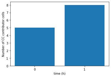
the total number of cluster = {0: 5, 1: 8}
As stated in the output above, at time_point = 0 we had 5 CC contributor cells, but at time_point = 1 we had 8.
We can plot the above result by using a function called plot_active_cell_all_time_point().
This function will takes the dictionary output of the get_count_cc_contributors_tp(). But before using the function, let’s import its library:
[23]:
import fitMultiCellSumStat.plot_sumstat as pss
[24]:
ax = pss.plot_active_cell_all_time_point(CC_Contributor_count_result)